ggplot2 extras

library(ggplot2)
library(palmerpenguins)

Project Defaults

Default themes

In a single document, if you want to have all of your plots have the same theme, you can set it with theme_set().

penguins |>
  ggplot(
    aes(
      bill_length_mm,
      bill_depth_mm,
      color = species
    )
  )+
  geom_point() -> p

penguins |> 
 ggplot(
    aes(
      bill_length_mm,
      bill_depth_mm,
      color = bill_length_mm
    )
  )+
  geom_point() -> p2

p + labs(title = "before")
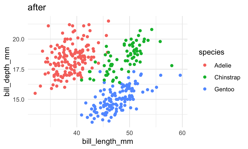
theme_set(
  theme_minimal()
)

p + labs(title = "after")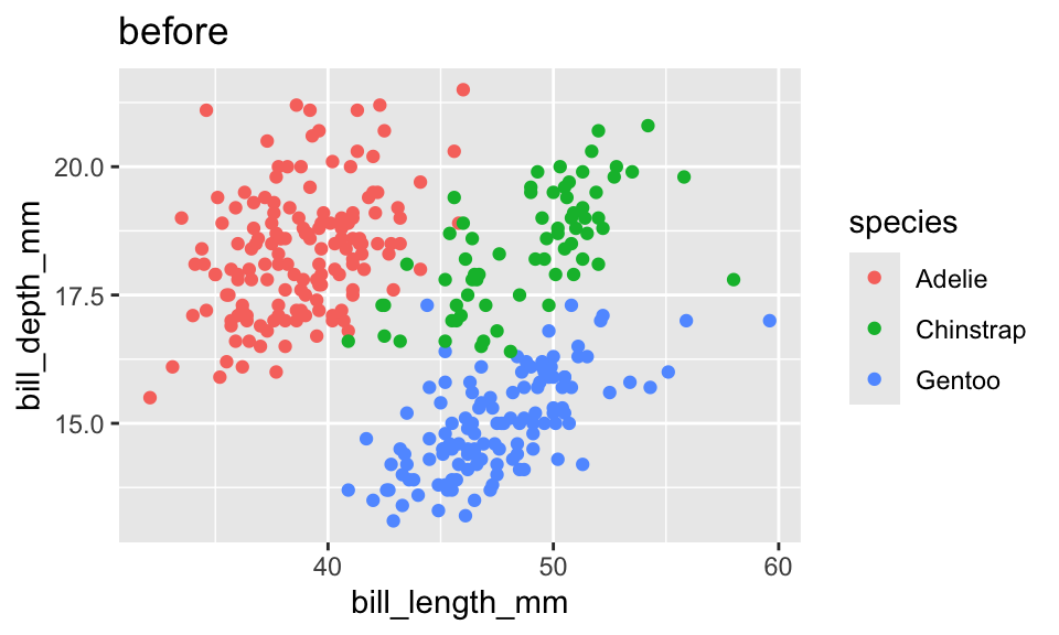

Default colors & fills

If you know you never want to use the default colors, adding the new color scale each time can get annoying:

library(ggthemes)
library(scico)

p+
  scale_color_ptol()+
  labs(title = "ptol")
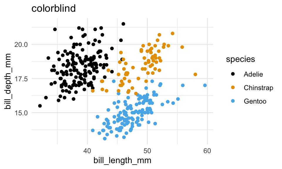
p +
  scale_color_colorblind()+
  labs(title = "colorblind")
p2 +
  scale_color_scico(
    palette = "batlow"
  )+
  labs(title = "batlow")
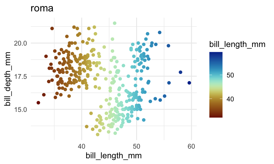
p2 +
  scale_color_scico(
    palette = "roma"
  )+
  labs(title = "roma")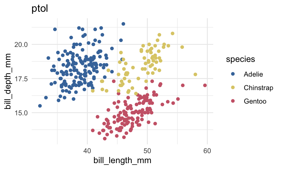

You can change the default color scales for all plots by setting some options()

options(
  ggplot2.discrete.colour = ggthemes::scale_color_ptol,
  ggplot2.discrete.fill = ggthemes::scale_color_ptol,
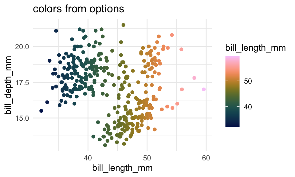
  ggplot2.continuous.colour = \(x) scico::scale_color_scico(palette = "batlow"),
  ggplot2.continuous.fill = \(x) scico::scale_color_scico(palette = "batlow")
)

p +
  labs(title = "colors from options")
p2 +
  labs(title = "colors from options")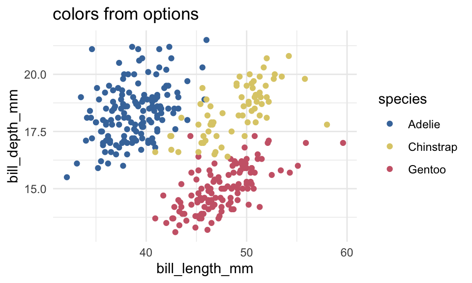

Multi-page defaults

I put the defaults I want to use across an entire project in an R script called _defaults.R and run all of that R code with source(), usually in a hidden code-chunk. You can look at the code of my _defaults.R here.

source(here::here("_defaults.R"))

p + labs(title = "after _defaults.R")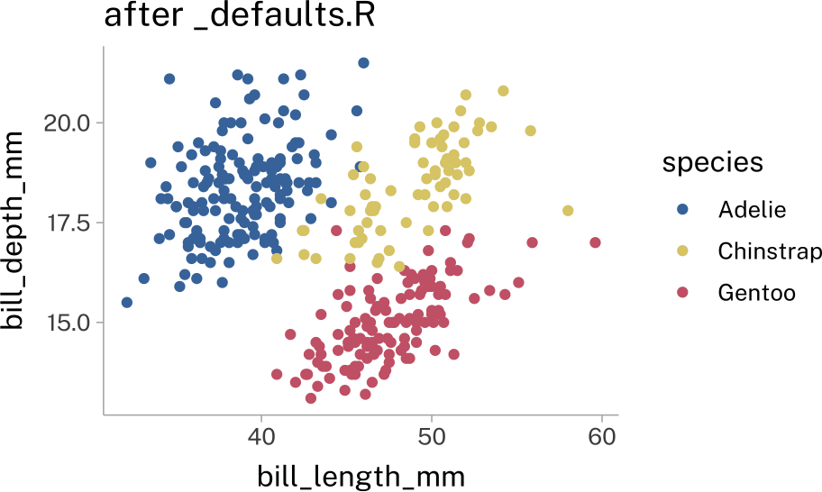

Direct labels

There are a two packages that are pretty useful for adding direct labels to plots

• ggrepel

• geomtextpath

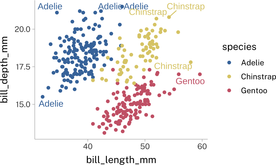
ggrepel

This will try to add labels to each point, and do as much work as possible to avoid labels overlapping.

library(ggrepel)

p +
  geom_text_repel(
    aes(
      label = species
    ),
    show.legend = F
  )

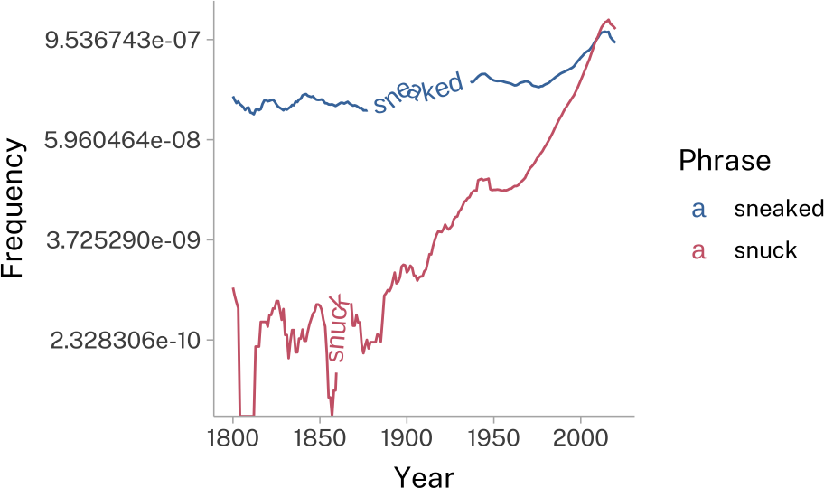
geomtextpath

This will add text along any given line element.

library(geomtextpath)
library(ngramr)

s_past <- ngram(c("sneaked", "snuck"))

s_past |> 
  ggplot(
    aes(
      Year,
      Frequency,
      color = Phrase
    )
  )+
  geom_textline(
    aes(
      label = Phrase
    )
  )->
  sneak_plot

sneak_plot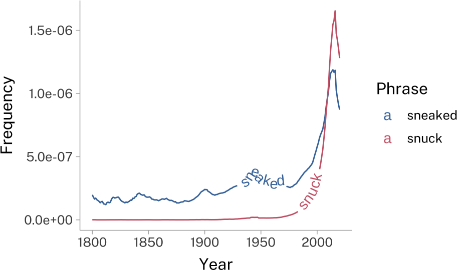

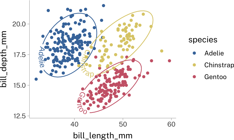
p + 
  stat_ellipse(
    geom = "textpath",
    aes(label = species),
    show.legend = F
  )

Axes

The expand argument

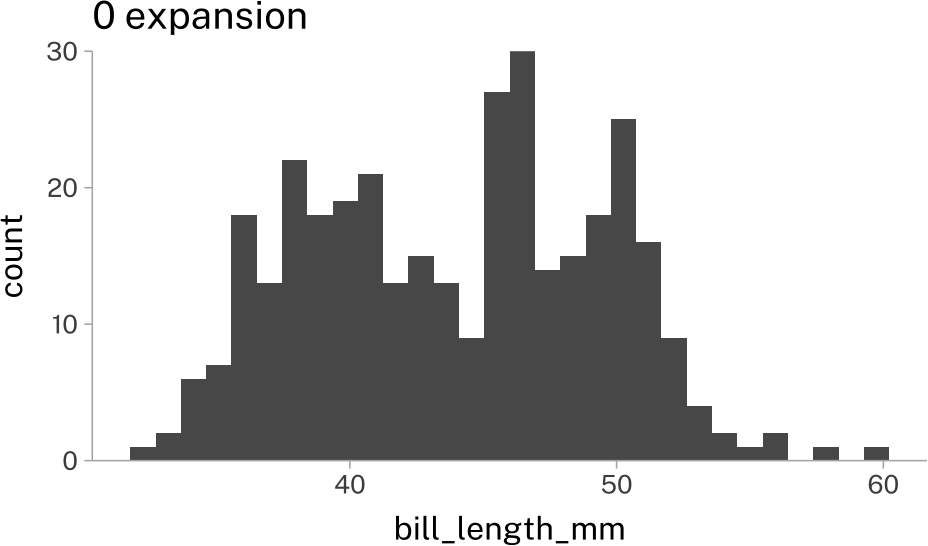
By default, ggplot will leave some “breathing room” on each axis. But if you want your pot elements to sit directly on the axes (this is nice for things like bars) you can mess around with the expand argument to the relevant scale.

penguins |> 
  ggplot(
    aes(bill_length_mm)
  )+
    stat_bin() ->
  hist_plot

hist_plot +
  labs(title = "default `expand`")
hist_plot +
  scale_y_continuous(
    expand = expansion(0)
  )+
  labs(title = "0 expansion")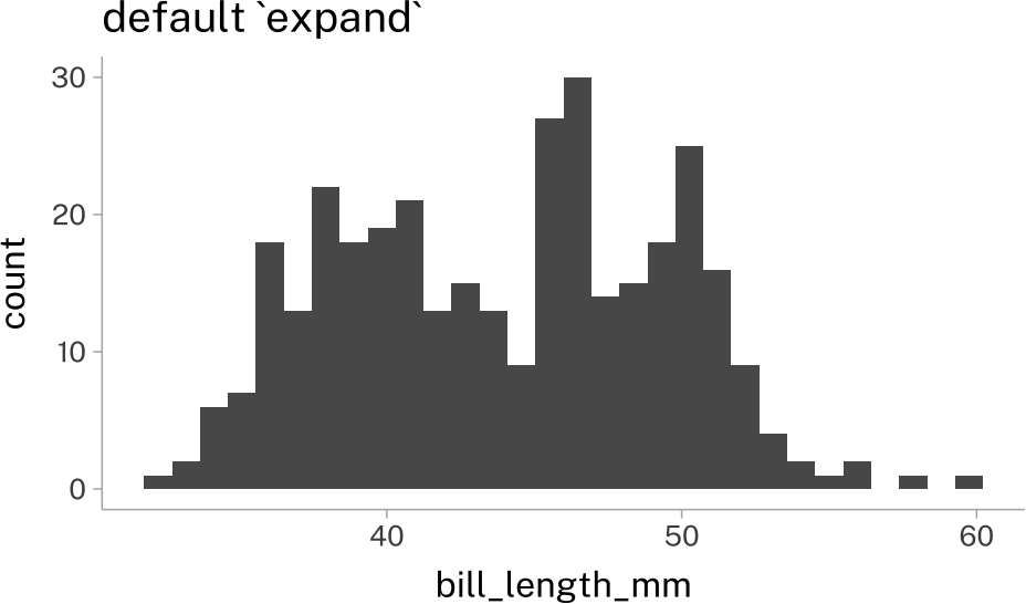

Custom Axes Transformations

The scales package lets you apply transformations to the plot axes.

library(scales)

sneak_plot +
  scale_y_continuous(
    transform = "log2"
  )

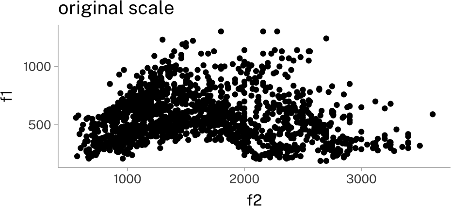
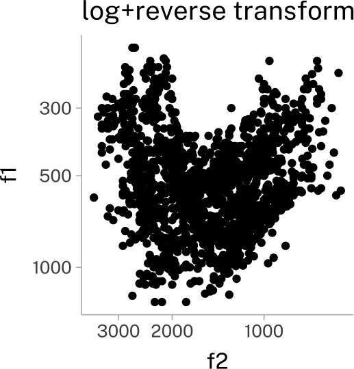
You can also define your own new transformations. This is useful for something like vowel formants, which we always want to reverse, and sometimes want to log transform.

library(phonTools)
data("pb52")

pb52 |> 
  ggplot(
    aes(
      f2,
      f1
    )
  )+
    geom_point()+
    coord_fixed()->
  vplot

vplot +
  labs(
    title = "original scale"
  )
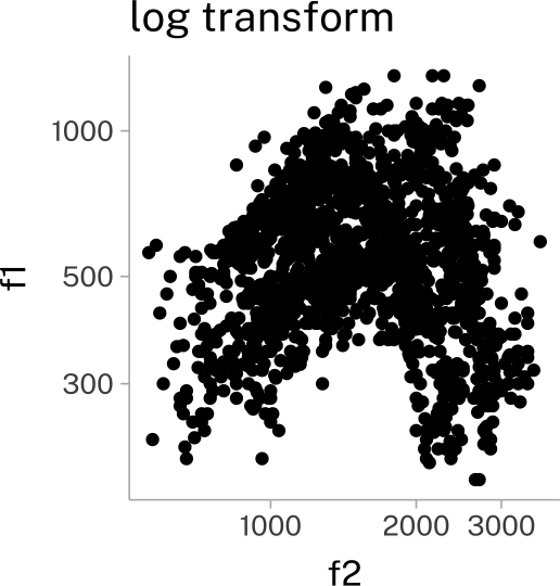
vplot +
  scale_x_continuous(transform = "log10")+
  scale_y_continuous(transform = "log10")+
  labs(
    title = "log transform"
  )
vplot +
  scale_x_continuous(transform = c("log10", "reverse"))+
  scale_y_continuous(transform = c("log10", "reverse"))+
  labs(
    title = "log+reverse transform"
  )

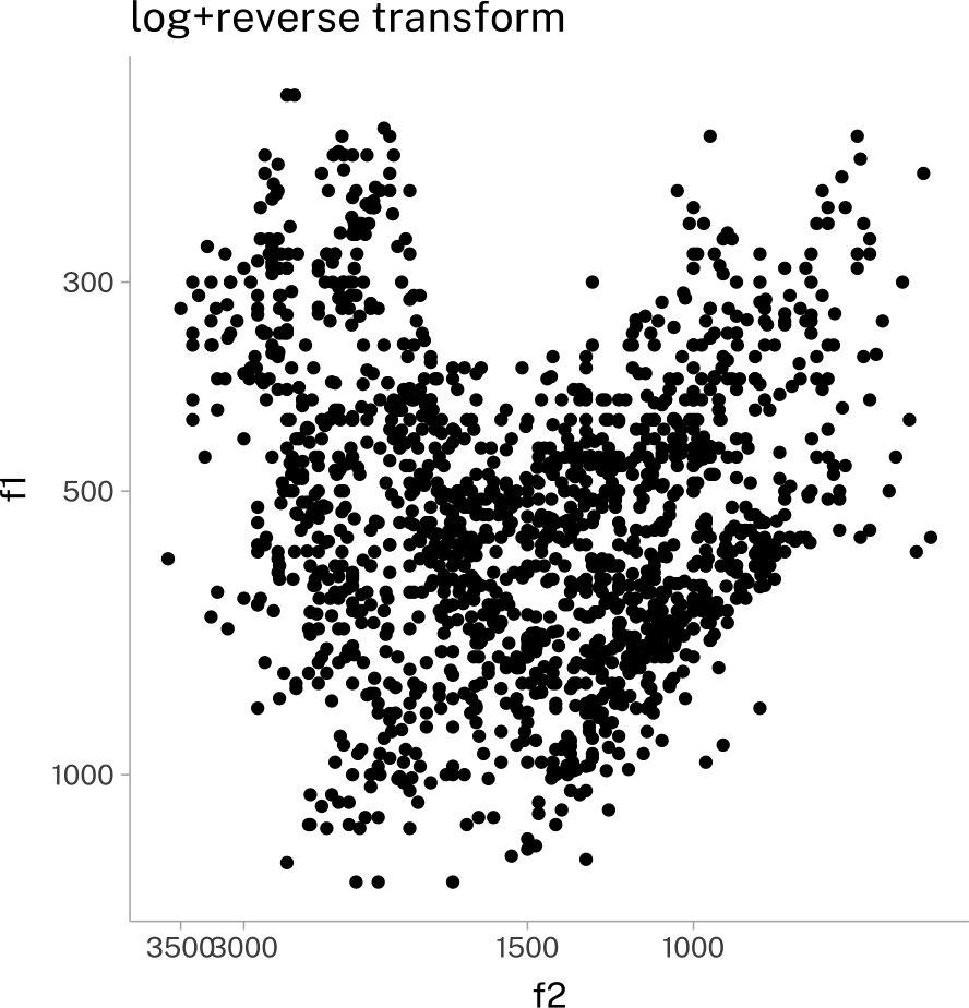
Scale breaks

Sometimes, you might want to customize which values are included in the axis breaks (although, ggplot is pretty good at setting these).

vplot +
  scale_x_continuous(
    transform = c("log10", "reverse"),
    breaks = c(1000, 1500, 3000, 3500)
  )+
  scale_y_continuous(transform = c("log10", "reverse"))+
  labs(
    title = "log+reverse transform"
  )

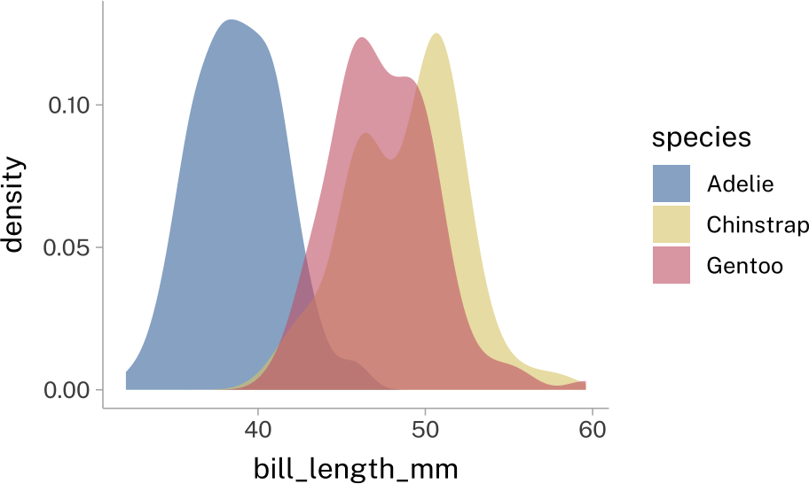
Overplotting

Sometimes you’ll deal with overlapping geometries. The most common way to deal with this is to set their transparency to something less than 1.

penguins |> 
  ggplot(
    aes(
      bill_length_mm, 
      fill = species
    )
  )+
    stat_density(
      position = "identity",
      alpha = 0.6
    )

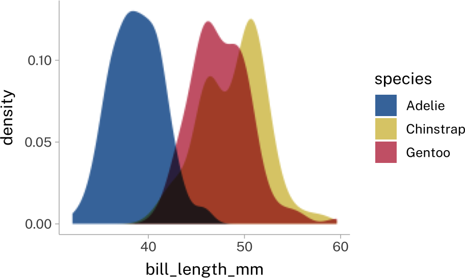
There’sa new-ish package called ggblend that can help with this, but they way it works can be a bit complex.

library(ggblend)

penguins |> 
  ggplot(
    aes(
      bill_length_mm, 
      fill = species
    )
  )+
    (
      stat_density(
        position = "identity"
      ) |>
        blend("multiply")
    )

ggdist

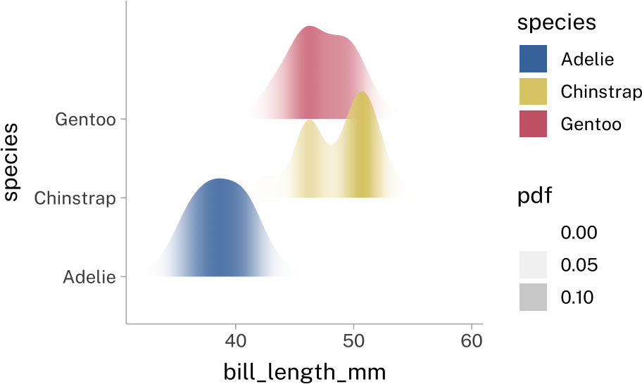
The ggdist package will come into play more when we start doing model visualization. For now, it’s sufficient to know it exists, and has a lot of cool features.

library(ggdist)

penguins |> 
  ggplot(
    aes(
      x = bill_length_mm,
      y = species,
      fill = species
    )
  )+
    stat_slab(
      aes(
        fill_ramp = after_stat(pdf)
      ),
      fill_type = "gradient",
      height = 1.5
    )+
    scale_fill_ramp_continuous(
      from = rgb(1, 1, 1, alpha = 0)
    )

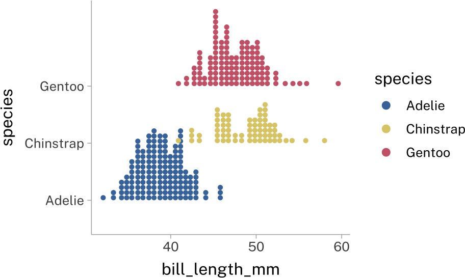
penguins |> 
  ggplot(
    aes(
      x = bill_length_mm,
      y = species,
      fill = species,
      color = species
    )
  )+
    stat_dots(
      height = 1.5
    )

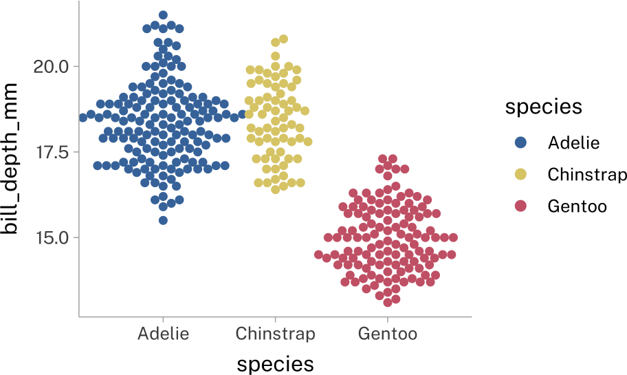
penguins |> 
  ggplot(
    aes(
      x = species,
      y = bill_depth_mm,
      fill = species,
      color = species
    )
  )+
    stat_dots(
      side = "both",
      layout = "swarm",
      width = 1.5
    )

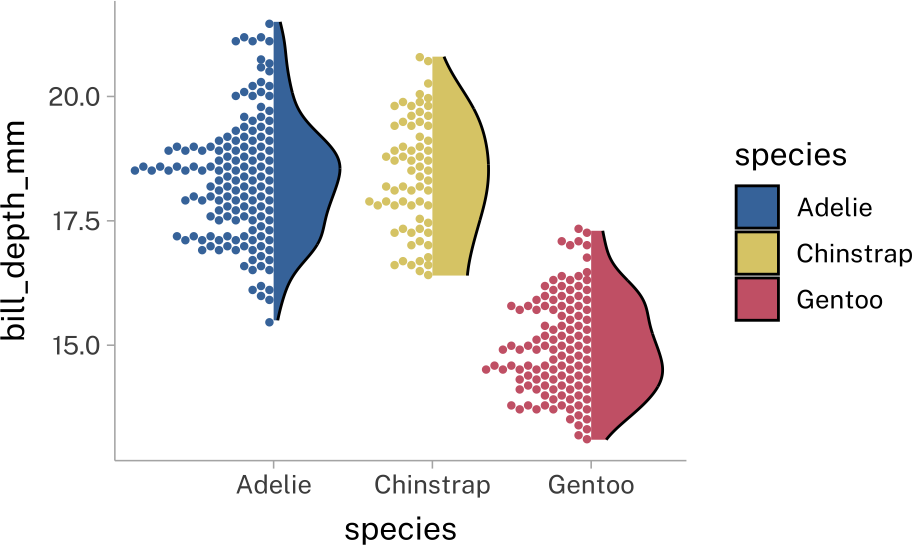
penguins |> 
  ggplot(
    aes(
      x = species,
      y = bill_depth_mm,
      fill = species,
      color = species
    )
  )+
    stat_slab(
      side = "right",
      color = "black",
      linewidth = 0.5,
      width = 0.5
    )+
    stat_dots(
      side = "left",
      layout = "hex"
    )