Pivoting Data

Data Setup

library(tidyverse)

remotes::install_github("jvcasillas/untidydata")

library(untidydata)
data("pb52", package = "phonTools")

Untidy data

Sometimes, we’ll create or encounter data that is “untidy.” Take something like pb52_wide.csv which you can read into R with:

pb52_wide <- read_csv("https://lin611-2024.github.io/notes/meetings/data/pb52_wide.csv")

head(pb52_wide)

This dataframe has 1 column for f0 through f3 for each vowel. This is not an outlandish kind of format to encounter! So, what to do?

Pivoting

By “pivoting” data, we take it from a wide to a long format, or vice versa. With the pb52_wide data, we still want f0 through f3 in the columns, but we want the vowel labels to be in the rows.

Step1: pivot longer

pb52_wide |> 
  pivot_longer(
    matches("f\\d"),
    names_to = "vowel_formant"
  )->
  pb52_long

head(pb52_long)

Equivalent approaches

pb52_wide |> 
  pivot_longer(
    cols = 5:44
  )

pb52_wide |> 
  pivot_longer(
    cols = i_f0:er_f3
  )

Step 2: Separate

Now, we want to split the vowel_formant column in two. Fortunately, the vowel name and the formant name are neatly separated by underscores. We can split them into separate columns with separate_wider_delim().

pb52_long |> 
  separate_wider_delim(
    vowel_formant, 
    delim = "_", 
    names = c("vowel", "formant")
  ) ->
  pb52_sep

head(pb52_sep)

Step 3: pivot wider

Now, we want to pivot wider, to get one column per formant. We can do this with pivot_wider().

pb52_sep |> 
  pivot_wider(
    names_from = formant,
    values_from = value
  )->
  pb52_tidied

head(pb52_tidied)

Applied Pivoting

There is at least one super common application for pivoting data longer and wider: vowel normalization. The “size” of speaker’s acoustic vowel space varies, and is usually inversely proportional to their height.

pb52 |> 
  ggplot(
    aes(f2, f1)
  )+
    geom_point()+
    scale_x_reverse()+
    scale_y_reverse()+
    facet_wrap(~type)+
    coord_fixed()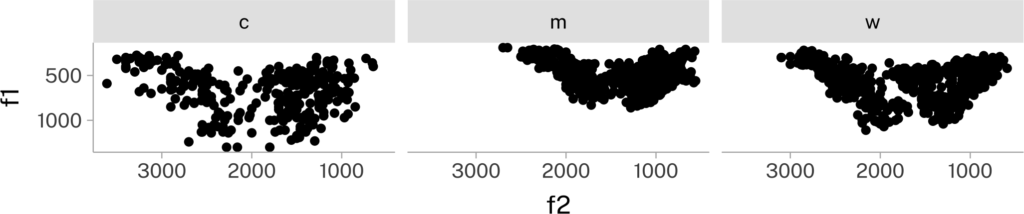

One way to “normalize” this is:

• For each speaker, apply the log transform to their f1 through f\(n\) data.

• For each speaker, get the average of all formant values.

• Subtract this average from all formant values.

The challenge

pb52 |>
  head()

It isn’t easy to get the average of f1 and f2 and f3 all together, while they are in separate columns.

The solution

We’ll use pivoting!

Pivot longer

Since we’ll want to come back to this same basic data arrangement, we’ll add a token_id column.

pb52 |> 
  mutate(
    token = row_number()
  ) |> 
  pivot_longer(
    f1:f3,
    names_to = "formant",
    values_to = "value"
  )->
  long_formants

head(long_formants)

Normalize with a grouped mutate

long_formants |> 
  mutate(
    .by = speaker,
    value = log(value) - mean(log(value))
  )->
  long_normed

head(long_normed)

Pivot back to wide

Now we can pivot back to wide for our normalized data.

long_normed |> 
  pivot_wider(
    names_from = formant,
    values_from = value
  )->
  pb52_normed

head(pb52_normed)

pb52_normed |> 
  ggplot(
    aes(f2, f1)
  )+
    geom_point()+
    scale_y_reverse()+
    scale_x_reverse()+
    facet_wrap(~type)+
    coord_fixed()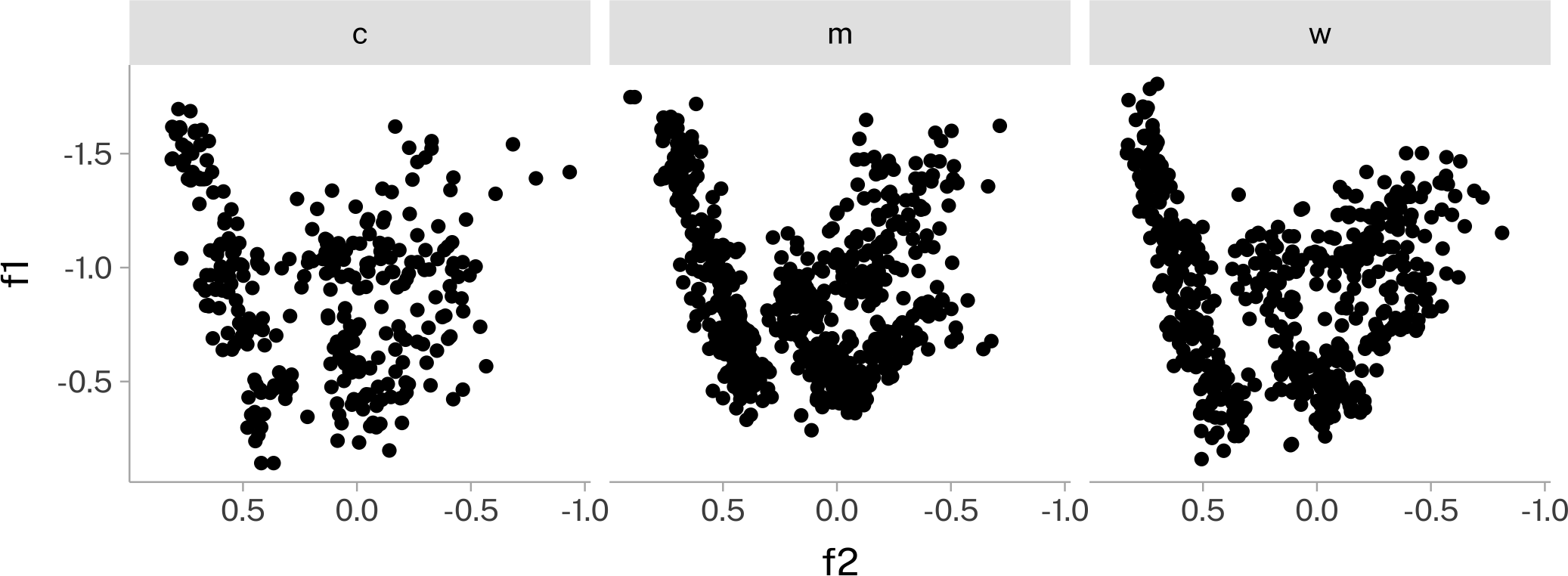

Exercise

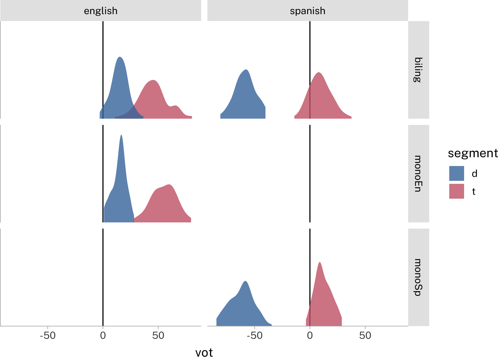
Take a look at the vot data from untidydata

head(vot)

Get the data into shape for making this plot: