Data Opertations in the Tidyverse

Data Frame Recap

library(tidyverse)
library(babynames)

Filtering

babynames |> 
  filter(name == "Josef") |> 
  head()

Summarising

babynames |> 
  summarise(
    total = sum(n)
  ) |> 
  head()

Filtering and Summarising

babynames |> 
  filter(
    name == "Josef"
  ) |> 
  summarise(
    total = sum(n)
  ) |> 
  head()

Mutating

babynames |> 
  mutate(
    name_length = nchar(name)
  ) |> 
  head()

Split-Apply-Combine

What if

What if we wanted a plot of how many total baby names there were each year?

We know how to get the total for 1 year with filtering and summarising.

babynames |> 
  filter(
    year == 1880
  ) |> 
  summarise(
    total = sum(n)
  )

But there a lot of unique years in the data

babynames |> 
  summarise(
    min = min(year),
    max = max(year)
  ) |> 
  mutate(
    total_years = (max-min)+1
  )

I don’t want to filter and summarise 138 times.

.by or group_by()

babynames |>
  summarise(
    .by = year,
    total = sum(n)
  )

1

This will group the day by year, then apply the summarising within each group.

The .by argument is really handy. There’s another way to write it out that explicitly uses a function called group_by()

babynames |>
  group_by(year) |>
  summarise(
    total = sum(n)
  )

1

This will group the data frame, then any subsequent data verbs will apply within the grouping.

Stretch Exercise

This goes one step further than what’s in the notes. Calculate the total number of baby names by year and sex.

Exercise

Hints

To summarise just by year, we passed a single column name to summarise()

babynames |>
  summarise(
    .by = year,
    total = sum(n)
  )

How do we construct a vector of values in R?

Solution

babynames |> 
  summarise(
    .by = c(year, sex),
    total = sum(n)
  )

More Split-Apply-Combine

Scenario

Oakley and Skyler are collaborating on a programming project, and for some reason they want to keep track of how many lines of code they contribute on each day.

tibble(
  day = c(
    "Monday", "Tuesday",
    "Monday", "Tuesday", "Wednesday"
  ),
  name = c(
    "Oakley", "Oakley",
    "Skyler", "Skyler", "Skyler"
  ),
  lines = c(
    10, 30,
     5,  5, 10
  )
)->
  collab_df

collab_df

1

This will be the day column.

2

This will be the name column.

3

This will be the lines column.

Query 1

Oakley wants to know, on each day, what proportion of lines they wrote.

collab_df |> 
  mutate(
    .by = day,
    day_lines = sum(lines),
    person_prop = lines/day_lines
  )

Query 2

Skyler wants to know how their contributions are distributed across days.

Exercise

Hint

This is still going to involve summing across the lines column.

Solution

collab_df |> 
  mutate(
    .by = name,
    total = sum(lines),
    day_prop = lines/total
  )

Joining

Oakley and Skyler have, for some reason, wanted to include their year of birth in the data frame. So they create a separate yob data frame.

tibble(
  name = c("Oakley", "Skyler"),
  year = c(2000, 1995)
)->
  yob

yob

To merge this yob data onto their colab_df data, they can use left_join().

collab_df |> 
  left_join(
    yob
  )->
  collab_df

collab_df

Exercise

Oakley and Skyler are having an argument about which name was more popular in their respective years of birth. They’ve made a total_babies data frame like this:

babynames |> 
  summarise(
    .by = c(year, name),
    total_babies = sum(n)
  )->
  total_babies

total_babies

How would they get the correct values for total_babies included as a column on collab_df?

Exercise

Hint

Don’t overthink this one.

Solution

collab_df |> 
  left_join(total_babies)

Practical Applications

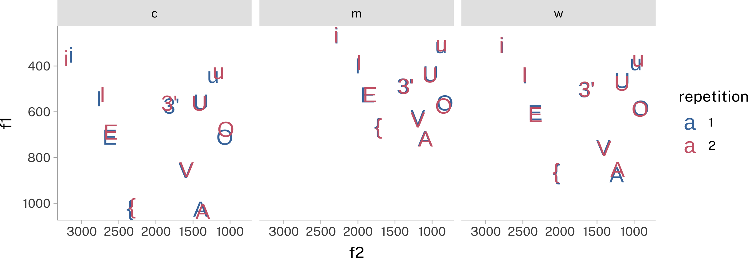
Case 1: A vowel means plot

The Peterson & Barney dataset

library(phonTools)

data("pb52")

head(pb52)

Let’s get the means for a plot

pb52 |>
  summarise(
    .by = c(type, repetition, vowel),
    across(f0:f3, mean)
  ) ->
  pb52_means

pb52_means

1

This across() function is handy way to apply the same operation (mean()) to a whole bunch of columns.

pb52_means |>
  ggplot(
    aes(
      x = f2,
      y = f1,
      color = factor(repetition)
    )
  )+
    geom_text(
      aes(label=vowel),
      size = 6
    )+
    scale_x_reverse()+
    scale_y_reverse()+
    facet_wrap(~type)+
    labs(
      color = "repetition"
    )+
    theme(
      aspect.ratio = 1
    )

1

I have to change the data type of repetition so it gets categorical data coloring, not continuous coloring.

2

While not accurate to the data spans, for now I want the plotting area of each facet to be square. That is the height:width ratio = 1

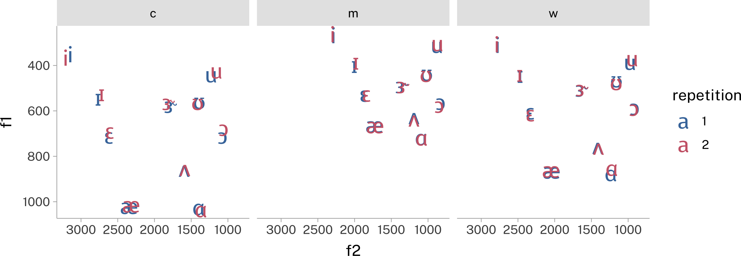
But, that X-SAMPA isn’t everyone’s cup of tea. Here’s a translation data frame from X-SAMPA to IPA (although, there is a package called {ipa}which might be able to do this easier).

tibble(
  vowel = c(
    "{", "3'", "A",
    "E", "i",  "I",
    "O", "u", "U",
    "V"
  ),
  ipa = c(
    "æ", "ɝ", "ɑ",
    "ɛ", "i", "ɪ",
    "ɔ", "u", "ʊ",
    "ʌ"
  )
)->
  vowel2ipa

vowel2ipa

1

These are the original labels in the data set.

2

These are the new IPA labels I want to use, which I just copy-pasted from an internet keyboard.

Now, you need to join the translation data frame onto the means data frame.

library(showtext)
font_add_google("Voces", "Voces")
showtext_auto()

pb52_means |>
  left_join(vowel2ipa) |>
  ggplot(
    aes(
      x = f2,
      y = f1,
      color = factor(repetition)
    )
  )+
    geom_text(
      aes(label=ipa),
      size = 6,
      family = "Voces"
    )+
    scale_x_reverse()+
    scale_y_reverse()+
    facet_wrap(~type)+
    labs(
      color = "repetition"
    )+
    theme(
      aspect.ratio = 1
    )

1

I needed to grab a font that could render the IPA symbols.

2

The crucial `left_join()`.

3

Setting the font family to be IPA ready.